Impact of transfer learning methods and dataset characteristics on generalization in birdsong classification

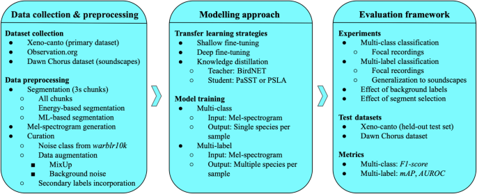
The data processing, methodology, and evaluation workflow for this study are outlined in Fig. 1.

Overview of the data processing, methodology, and evaluation pipeline.

Transfer learning

Transfer learning is a machine learning technique where knowledge gained from one domain is applied to another domain. “Knowledge” here is a shorthand term to express that a trained system has stored latent information about how to extract general or specific information from its input data, based on the training data’s characteristic patterns and distributions. The approach leverages a model developed for one task as a starting point for another, related task, often compensating for limited or inadequate data in the destination domain¹⁷. The primary idea is to utilize the patterns learned from a large dataset in the source domain and fine-tune them to improve performance on a different but related problem in the target domain. In the context of deep learning, transfer learning most commonly involves using a pre-trained network (trained on a large dataset such as ImageNet or AudioSet) and finetuning it on a smaller, task-specific dataset. Note however that there can be many ways to achieve transfer learning. For example, Ntalampiras (2018) extracted features from a (non-deep) classifier trained on music, as input to a bird classifier²⁹.

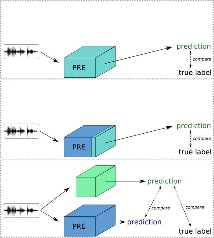
Transfer learning strategies. Light-coloured blocks are neural networks being trained; dark-coloured blocks are ‘frozen’ and unchanging during transfer learning. Deep finetuning (top) retrains all layers. Shallow finetuning (middle) uses most of the pretrained model as a fixed feature extractor, retraining the final layer(s) on the new dataset. Knowledge distillation (lower) differs from both of these, training a new model to produce the same outputs as the teacher model, and also to match ground-truth labels when they are available.

Birdsong classification is a challenging task due to the limited availability of labeled bird sound recordings and the complexity and variability of bird vocalizations. Transfer learning is particularly useful in this context for several reasons. First, data scarcity is a common issue, as birdsong datasets are often small and imbalanced. Transfer learning allows us to leverage pre-trained models that have been trained on large datasets, mitigating this problem. Second, these pre-trained models have learned to extract rich features that capture important patterns and characteristics in audio signals, which can significantly enhance the accuracy of birdsong classification. Additionally, starting with a pre-trained model reduces the time and computational resources needed to train a model from scratch, as the initial layers already contain useful representations. In this study, we explore different transfer learning strategies, including deep finetuning, shallow finetuning, and knowledge distillation, to capitalize on the advantages of using pre-trained models for birdsong classification. These strategies not only address data scarcity and improve feature richness but also streamline the training process, making transfer learning particularly beneficial for this task.

We next describe the transfer learning strategies considered in the present work.

Deep finetuning

Deep finetuning involves adjusting all layers of a pre-trained model on a specific dataset, in this case, the birdsong dataset. This comprehensive adjustment enables the model to better capture and adapt to the unique characteristics of bird sounds, adapting its “early” and “late” processing stages and thus potentially improving its performance on this specialized task. However, this approach has two potential drawbacks. Retraining the entire network may be computationally costly, especially as larger and larger networks are introduced. The method also risks overfitting to the new dataset, since there are many free parameters: if all layers are free to change, the pretrained knowledge may be fully erased by the later training, a phenomenon referred to as “catastrophic forgetting”^30,31. To mitigate this, deep finetuning needs careful implementation and/or a relatively large dataset.

The optimisation for deep finetuning is the same as for ordinary training of a deep neural network, in which we define a loss function L dependent on the input (spectrogram) X and the ground-truth label y:

Here \(L_g\) is a standard loss function such as cross-entropy, and f representing the neural network. The final nonlinearity of the neural network is shown explicitly as the function \(\delta\), which we will later refer to, separately from the unnormalised outputs (“logits”) of f. The parameters of f (not shown) are chosen to minimise L.

In the context of deep learning, finetuning pre-trained models has been shown to yield significant improvements in various tasks. For instance, Howard and Ruder³² demonstrated that finetuning the entire model, as opposed to only the final layers, can result in substantial gains in performance on text classification tasks . Similarly, in the field of computer vision, deep finetuning of convolutional neural networks (CNNs) has been proven effective in adapting models to new domains, as evidenced by Yosinski et al.³³, who highlighted the benefits of finetuning across different tasks and datasets .

Moreover, recent advancements in finetuning techniques, such as those described by Raffel et al.³⁴ in their work on the T5 model, underscore the importance of appropriately scaling the model and dataset size to achieve optimal results. Applying these principles to the task of birdsong recognition, deep finetuning has the potential to harness the power of pre-trained models to enhance performance, provided that sufficient data and computational resources are available to support the process.

Shallow finetuning

In shallow finetuning, only the final layers of a pre-trained model are adjusted to fit on the target dataset, while the early layers remain unchanged. The unchanged part of the pre-trained model can be considered as a feature extractor, providing a rich set of learned features that should be useful for the new task. This method is less computationally intensive compared to deep finetuning, since only a small/shallow part of the network needs to be trained. It can be particularly effective when working with smaller datasets, as it is strongly constrained to leverage the general features previously learned by the lower layers of the model.

To express shallow finetuning mathematically, we separate the network f into two parts:

where \(f_1\) is constant, and the parameters of \(f_2\) are optimised.

Shallow finetuning has been demonstrated to be effective in various contexts. White et al.³⁵ showed that adapting trained CNNs to new marine acoustic environments by only finetuning the top layers allowed the models to effectively generalize to different conditions without extensive retraining . This strategy not only saves computational resources but also reduces the risk of overfitting, making it suitable for tasks with limited data.

Additionally, Ghani et al.¹² highlighted the benefits of using global birdsong embeddings to enhance transfer learning for bioacoustic classification. By leveraging pre-trained embeddings and finetuning only the top layers, their approach achieved superior performance with minimal computational overhead. Similarly, Williams et al.³⁶ emphasized the advantages of using pre-trained models on diverse sound datasets, including tropical reef and bird sounds, to improve transfer learning in marine bioacoustics. Their work supports the efficacy of shallow finetuning in adapting models to new acoustic environments .

These studies underscore that shallow finetuning can effectively utilize the robust, general features captured by the lower layers of pre-trained models, making it a practical and efficient approach for tasks like birdsong recognition, especially when computational resources and dataset sizes are limited.

Knowledge distillation

Knowledge distillation is a technique where a pre-trained model is not itself changed: instead, it acts as a “teacher” and guides the training of a student model (Fig. 2, lower panel). In doing so the knowledge is transferred to the student model, to obtain a competitive performance versus the teacher model^25,26. This is often applied by training the student on “soft targets” from the teacher model: the fuzzy predictions rather than binarised 1-or-0 decisions. We interpret this as training the student to approximate the continuously-varying prediction function that the teacher outputs.

While model compression for efficiency and speed is a significant motivation behind this process, i.e. training smaller models from large²⁷, improved generalization and transfer learning are also key benefits. Learning from the nuanced information in the teacher’s soft targets helps the student model to learn the rich similarity information between classes that the teacher model has established^26,37. Interestingly, recent research has shown that cross-model distillation between different architectures, such as convolutional neural networks (CNNs) and transformer models, can yield superior performance, leveraging the strengths of both types of models to create a more robust and effective student model³⁸. This can be interpreted as one model learning to approximate information encoded not only in the data, but also in the biases implicit in the architecture of a very different network.

The original knowledge distillation framework was proposed by²⁶. Although diverse and more complex attention distillation techniques have since been studied³⁹, the authors in³⁸ reported that the original method is more effective, provided that certain details such as “consistent teacher” training are used⁴⁰. Therefore, we employ this approach. During the training of the student model, we use the same input with “consistent teaching”, meaning that the teacher and student are exposed to identical mel spectrograms, even when data augmentation is used to modify the training data. To train the student model the following loss is minimized, composed of two parts³⁸:

The coefficient \(\lambda\) represents the weighting whose value, following³⁸, we fix at 0.5. The terms \(\text {L}_g\) and \(\text {L}_{kd}\) correspond to the ground truth and distillation losses, respectively. In other words, the knowledge distillation can be seen as a weighted sum of ground truth loss \(\text {L}_g\) and distillation loss \(\text {L}_{kd}\). The symbol \(\delta\) denotes the activation function, while \(f_s\) and \(f_t\) are the student and teacher models, respectively. The parameter \(\tau\), referred to as the “temperature,” is set to \(\tau\) = 1.0 in alignment with³⁸, which showed that using this value yields optimal results for knowledge distillation when a CNN serves as the teacher and a transformer acts as the student. It is important to note that the teacher model remains frozen during the training of the student model.

We employ the cross-entropy (CE) loss as \(\text {L}_g\), combined with the softmax activation function, for multi-class classification (single-label AvesEcho v0). For the multi-label classification (AvesEcho v1), we utilize the binary cross-entropy (BCE) loss as \(\text {L}_g\) with the sigmoid activation function. Additionally, we use Kullback-Leibler divergence as the knowledge distillation loss \(\text {L}_{kd}\) for multi-class classification, and binary cross-entropy (BCE) loss for multi-label classification.

Audio data

To build a model allowing for the monitoring of European breeding birds we selected species in the 2nd European Breeding Bird Atlas (EBBA2)⁴¹ identified as breeding in Europe. This also includes all birds normally wintering or migrating in our target geography (running up to the Ural in the east). This list includes all birds found breeding in Europe in the period 2013-2017 including established non-native species.

Geographic distribution of our data sourced from Xeno-canto.

We then downloaded corresponding audio data from Xeno-canto⁴², the citizen-science open data source for animal sound recordings. We used the Xeno-canto API to select sound recordings preferentially of high quality, and recorded in Europe. Xeno-canto (XC) is the largest open access database of nature sounds and available recordings cover all European breeding birds, although for some very rare species the number of recordings is limited. Xeno-canto has the benefit that the overall quality of recordings is good and the identification is reliable due to peer-review by other workers. A further advantage is that the data is largely open access so that future models can make use of the same source of training data.

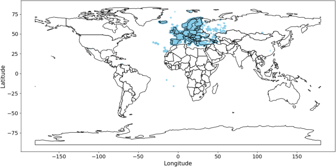
In the following we report on two studies of neural networks, based on slightly differing datasets. First, multi-class classification, based on the assumption that only one foreground bird is active. To achieve a minimum requirement of at least 10 recordings per species in order to train the recognition algorithm, we curated a list of 438 bird species for the multi-class model (AvesEcho v0). Second, to train a multi-label model in which multiple species can be simultaneously active, we relaxed the selection criteria to include more species from the EBBA2 list, and also to include recordings from outside Europe for species where we did not have enough recordings. Additionally, we added recordings from outside Europe for all species with less than 50 recordings to make the total for a species up to 50. This curation resulted in a list of 585 species for the multi-label model (AvesEcho v1). Fig. 3 shows geographical distribution of the data sourced from Xeno-canto for the multi-label model.

For both of these datasets, a noise class is included, which is derived from the warblrb10k dataset⁴³, specifically from the subset labeled as “0” indicating “no birds present,” and so consisting just noise.

Additionally, we also curated a dataset of 406 species from Observation.org⁴⁴ to test our single-species models on recordings from a source other than Xeno-canto.

Histogram depicting the number of labeled species within 3-second chunks from the Dawn Chorus dataset, illustrating the degree of polyphony present.

We also present results using a Dawn Chorus dataset developed by the Dawn Chorus project⁴⁵, a Citizen Science and Art initiative by the Naturkundemuseum Bayern/BIOTOPIA LAB and the LBV (The Bavarian Association for the Protection of Birds and Nature). The recordings were mostly short smartphone-based soundscapes collected during the dawn chorus – a time when many birds are most vocally active – by a worldwide community of enthusiasts. The dataset used in this study is a collection of 1-minute bird vocalisation recordings annotated by volunteers, including both professional and lay ornithologists. Only annotations from volunteers who scored 70% or higher on a species recognition questionnaire were included to ensure a high level of accuracy. The dataset comprises 236 annotated recordings from Germany, selected from a large worldwide pool of recordings⁴⁶ made available through the Dawn Chorus project. Annotations are conducted in 3-second chunks, following the BirdNET scheme, and are based on species identification through audio cues. The recordings in the dataset are primarily in uncompressed WAV format, although other formats like MP3 and FLAC are also present, particularly from earlier collection efforts. This subset represents a diverse range of bird species from Germany. Each recording in the dataset is linked to additional metadata, such as location and environmental conditions, though these were not utilized in the current analysis.

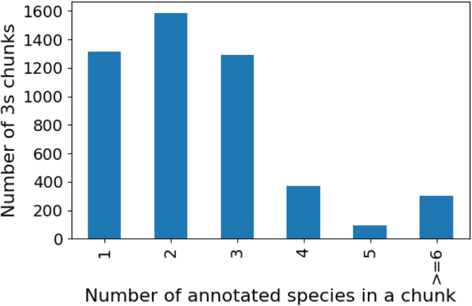
Table 1 provides a summary for different datasets used in this work and Fig. 4 shows a histogram illustrating the polyphony present in the Dawn Chorus dataset.

Challenges with Xeno-canto data for model training

While Xeno-canto offers significant advantages, such as being the largest open-access database of nature sounds, covering all European breeding birds, and providing high-quality, peer-reviewed, and reliable identifications, there are several challenges when using this data for training machine learing models.

(Left) Distribution of the number of recordings per species in the Xeno-Canto dataset for multi-label case. The plot shows that the distribution is unbalanced. (Right) Distribution of the total number of species annotated per file in our Xeno-canto data. The large peak at 1 indicates that many sound files are annotated as having no other species audible in the background.

Firstly, the data is weakly labelled: while the species of the vocalizing bird is known, the exact timing of these vocalizations within the recordings is not, complicating segment-based model training. Secondly, many background species are missing in the annotations, potentially impairing the detection of background vocalizations. This arises from Xeno-canto’s history, with its original design allowing only for one species per file. For machine learning this is a type of label noise: since many occurrences are in effect mislabelled as absences, it can bias a learning algorithm against making correct positive predictions. Thirdly, Xeno-Canto recordings are primarily focal recordings, designed to capture a target bird’s sound as clearly as possible, making these vocalizations louder and more prominent than those typically found in soundscapes. This discrepancy poses difficulties in recognizing fainter bird sounds. Finally, the dataset is limited for certain species, such as Stercorarius pomarinus and Puffinus mauretanicus, which have very few recordings available. Fig. 5 illustrates the distribution of the number of recordings per species within the dataset curated to train the model. This distribution highlights the variability in the amount of available data across different bird species. This scarcity necessitates either the removal of these classes or the collection of additional data to ensure accurate classification.

Despite these limitations, Xeno-canto powers most general-purpose birdsong classifiers, and this yields better bioacoustic recognition than models trained on more generic audio data such as AudioSet ¹². In the present study we aimed to evaluate how to make best use of the characteristics of Xeno-canto data, including the possible use of background labels.

Pretrained models

BirdNET⁸ utilizes EfficientNet, a well-established CNN architecture. It has been trained on an extensive dataset that includes recordings from Xeno-canto (XC), the Macaulay Library, and labeled soundscape data from various global locations, enabling it to recognize many thousands of bird species. Beyond avian identification, BirdNET is also capable of identifying human speech, dogs, and numerous frog species. This broad training set allows BirdNET to be highly versatile, supporting a range of downstream applications. To achieve this versatility, BirdNET strikes a balance between accuracy and computational efficiency, ensuring it can be deployed on a variety of devices with limited processing power. In this work, we report on BirdNET version 2.2, which offers improved performance and broader species coverage. The BirdNET codebase, along with comprehensive documentation, is publicly available on GitHub⁴⁷, facilitating further research and development in bioacoustic monitoring and related fields.

PaSST²¹ leverages the strengths of transformer architectures for audio classification. The model, similar to the AST⁴⁸, is inspired by the Vision Transformer (ViT)⁴⁹. It extracts patches from the spectrogram, adds trainable positional encodings, and applies transformer layers to the flattened sequence of patches. Transformer layers utilize a global attention mechanism, which causes the computation and memory requirements to increase quadratically as the input sequence lengthens³⁷. PaSST attempts to mitigate this by introducing an innovative training technique known as “Patchout,” which selectively drops patches of the spectrogram during training, enhancing efficiency and robustness. In this way, the model significantly reduces compute complexity and memory requirements for training these transformers for audio processing tasks. The model is competitive with SOTA and obtains a mAP of 47.1 using their best single model on the AudioSet-2M. The implementation of PaSST, along with its training framework and performance benchmarks is available for public access on GitHub⁵⁰.

PSLA²⁰ is an EfficientNet model trained on AudioSet. We include this model to have a comparison with the BirdNET model which employs the same CNN-based architecture. By pretraining on large-scale audio datasets, PSLA captures a wide range of audio features, which are further refined through strategic sampling and labeling processes. To generate predictions, it uses an attention layer on the final embeddings, distinguishing it slightly from BirdNET, which uses a single dense layer for the same purpose. The model is again competitive with SOTA and obtains a mAP of 44.3 using their best single model on the AudioSet-2M. In this work, PSLA is incorporated into our pipeline as simply a model pre-trained on AudioSet, and we apply finetuning after our own pre-processing steps, rather than using the pre-processing pipeline followed in the PSLA paper. The PSLA framework, along with its implementation details and performance metrics is documented and accessible for public access on GitHub⁵¹.

Data preprocessing

For our experiments, we used two different configurations for generating mel-spectrograms, tailored to the requirements of the PaSST and PSLA models. For the PaSST configuration, we used 128 mel bands, a sampling rate of 16,000 Hz, a window length of 400 samples, a hop size of 160 samples, and an FFT size of 512. With a 3-second input signal, these settings result in a mel-spectrogram with 298 time frames. For the PSLA configuration, we used 128 mel bands, a sampling rate of 32,000 Hz, a window length of 800 samples, a hop size of 320 samples, and an FFT size of 1024. Similarly, a 3-second input signal with these settings also results in a mel-spectrogram with 298 time frames. Both configurations ensure that the mel-spectrograms have the same number of time frames, facilitating a consistent comparison between the models. Unlike PaSST and PSLA, BirdNET includes a pre-processing stem (a spectrogram layer). For BirdNET, the data is fed as an audio time series with a fixed input size of 3 seconds, using a sampling rate of 48,000 Hz.

Additionally, we also experimented with various data augmentation techniques to improve model robustness and performance. After evaluating several options, we found that two augmentations provided the best results: MixUp⁵² and background noise addition. Both of these augmentations are applied directly to the raw waveforms before spectrogram conversion.

MixUp is a data augmentation technique where two samples are combined to create a new synthetic sample. We apply MixUp with a probability of 0.6, meaning that 60% of the time, two random samples are mixed together to create a new training example. A value lam is sampled from a Beta distribution to linearly combine two input samples and their labels, ensuring smooth interpolation between them rather than a hard selection, with lam controlling the ratio of the mix. Since the process operates in floating-point format, there is no risk of clipping during training. Additionally, no explicit SNR is controlled for mixup, as the relative contributions of the two signals are determined by lam.

For background noise addition, we augment the input sample by mixing them with noise samples with a probability of 0.5. In this way, a random half of training samples are mixed with noise. Background noise is scaled dynamically to a random SNR sampled from [3 dB, 30 dB]. This ensures variability while maintaining the original signal’s intelligibility. The augmentation is applied dynamically (“on-the-fly”) with a probability, and clipping is inherently avoided in floating-point processing. The noise samples are derived from the warblrb10k dataset, which contains a variety of background sounds, ensuring that the model becomes more resilient to environmental noise and can better generalize to real-world conditions.

The probability values for both MixUp and background noise were manually tuned in pilot testing. By incorporating these augmentations, we aim to enhance the models’ ability to generalize, ultimately leading to more robust performance across different acoustic environments.